Parallel Poisson Solver Example

Learning Objectives

At the end of this class, you should be able to:

1. Discretize and solve a simple elliptic PDE
2. Define the initial and boundary conditions to the problem
3. Implement a distributed memory parallelization
4. Describe the typical workflow for HPC computations

Time to complete: 60 min

Two-dimensional heat conduction problem

In this section we will solve a practical problem using parallel computing. Say your task is to study heat conduction in a square plate, in a two-dimensional space in a steady state, in which all four sides are at different temperatures and a heat source is located at the centre of the domain. As you may recall, this problem is mathematically described by the Poisson equation:

where is the temperature, which is a function of the two spatial dimension, is the Laplacian operator defined as , is the heat source, and is the thermal conductivity of the medium. This is one of the most important partial differential equations in physics and, due to its elliptical character, has some unique challenges in solving in parallel. The solution of elliptic PDEs depends uniquely on the values at the boundaries and the sources in the domain. For CFD applications, the Poisson equation is particularly important as the PDEs describing fluid motion, the well known Navier-Stokes system of equations, has elliptic characteristics, particularly in its incompressible formulation. Thus, a Poisson equation must usually be solved, and depending on the solution method, this one of the most expensive steps in the CFD calculation. Although the above equation could be solved analytically, we focus on its numerical solution.

Be careful

Solving the equation above numerically will only asymptotically tend towards the analytical solution. The discretized solution of the equation will give an approximation of the analytical solution.

This lesson is meant to provide an overview of the solution procedure; therefore the intricate details of the numerical methods will not be covered. Instead, we refer the interested reader to CFD Python: 12 steps to Navier-Stokes for additional information on the numerics used herein.

For the solution of the above PDE, we take the following steps:

1. Discretize the spatial domain
2. Transform PDE to algebraic ODE
3. Define boundary conditions
4. Solve the algebraic equation until convergence

Domain discretization

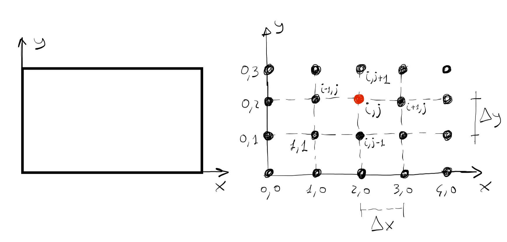
In this first step, we discretize the plate by dividing up the domain into a set of discrete grid points. Here, out of simplicity, we will assume that the grid points are equally spaced in both directions, thus we define the spacing between then by and . Given the simplicity of the Cartesian discretization grid (we will define the structured grid in the next section), we can identify every grid point in the domain by a pair of indices . Therefore the variable temperature at a grid point (red dot in the figure below) will be labeled as .

Domain discretization

This process can be thought of as the grid generation step. This step is not trivial in general and can be computationally very expensive depending on the size and complexity of the geometry. In our illustrative case, we have 6 interior grid points and 14 boundary grid points.

Transform PDEs to algebraic equations

The original equation that governs the physics of the problem is a second-order partial differential equation of the form:

Many techniques are used to discretize the governing equations, and entire textbooks are devoted to the theory behind it. Here we use the very easy finite difference method to write the PDE as a set of finite differences:

One can then rearrange the above equation to find the value of temperature at each grid point :

where . Note that refers to the temperature value at a nodal location, and therefore to solve the equation above and calculate we need the knowledge of the temperature at every neighboring point. In numerical analysis this is often referred to as a 4-points stencil problem.

Apply boundary conditions

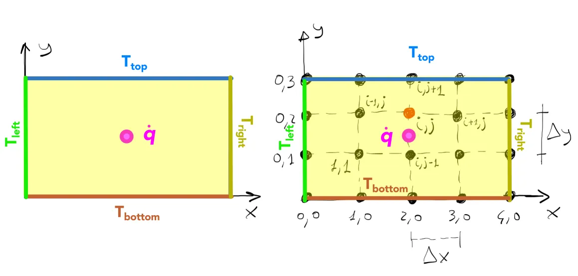
As the PDE corresponds to a boundary-value problem, the temperature values at the boundaries need to be provided in order to solve the governing equation. We consider that the rectangular plate is subject to a constant temperature boundary condition (Dirichlet) and has a heat source (input units in ) at the centre as shown in the figure below.

Boundary conditions of the rectangular plate.

In this very simple case, the temperature is set on all sides of the domain. Since many grid points are located on the boundary, the temperature of these grid points are known. Following the schematic figure above, one might say:

Given the four point stencil used in the problem, the corner points do not need to be defined as they do not enter into the solution of the interior points.

Solve the system of linear equations until convergence

The solution of the set of discretized governing equation can be represented by a linear system of equations of the form:

Where is a sparse matrix the size of which is related to the number of unknowns in our problem, is the variable field (in our case temperature), and is the right hand side (RHS). Because the temperature at the boundary grid points is known (boundary conditions) the system of linear equations must be solved for the interior points. Several techniques are described in the literature, however they mostly belong to two classes:

1. Direct methods: such as the Gauss-Jordan elimination method based on matrix inversion technique
2. Iterative methods: such as the Gauss-Seidel method or Jacobi iterative method

In this example we use the Jacobi iterative method. The solution to the linear system of equations will give us the temperature at all internal grid points and therefore the desired temperature profile across the plate.

If an iterative method is used to solve the linear system of equations, a convergence criterion must be chosen to STOP the iteration loop. In this very simple case, as the governing equations admit an analytical solution, we could define a convergence criterion based on the error from the exact solution. However, in most general cases, the governing do not admit an analytical solution.

The most common technique to monitor iterations, and ensure that convergence is reached is by checking the residual. Once the -th iteration has been computed we can define the residual as:

Where is the approximate solution at the -th iteration. To have a measure of the residual comparable at different mesh resolutions, the norm is often used as a more accurate parameter:

Parallelization strategy

As mentioned earlier, the matrix could be very large depending on our grid size, thus finding an approximate solution with a numerical method on a single processor can be very time consuming. Therefore, one should take advantage of the parallel computing strategy and exploit the capabilities of modern computer clusters.

In the following, we provide a parallelized code, written in the Python programming language, to solve the 2D Poisson equation as described above. Learners without a basic knowledge of Python should consider the following a tutorial. In the code, the user specifies the following input parameters (highlighted in grey in the code below):

1. Size of the domain: x_length, y_length.
2. Number of interior grid points: x_node, y_node.
3. Boundary conditions: T_top, T_right, T_bottom, T_left.
4. Strength of the source : Q_source
5. Thermal conductivity : therm_cond
6. Maximum number of iterations: iterations
7. Tolerance for the convergence check: epsilon

The parallelized code can be downloaded from the accompanying ARC4CFD git repository or copied from below. This code can be run on the HPC clusters or locally. The parallelization is achieved by using a distributed memory architecture with a message passing interface (MPI).

Click HERE to see the code

heat_conduction_mpi.py

####   Jacobi Iteration of Steady Heat Conduction equation Using MPI    #######

##  A rectangular domain with fixed boundary temperatures, is subject to
##  heat source at centre of the domain

import time
from mpi4py import MPI
import numpy as np
import matplotlib.pyplot as plt


def split_rows(rows, size):
#ref: https://stackoverflow.com/questions/55465884/how-to-divide-an-unknown-integer-into-a-given-number-of-even-parts-using-python
#This function splits the rows into near equal parts
    avg_rows, remainder = divmod(rows, size)
    lower = [avg_rows for i in range(size - remainder)]
    higher = [avg_rows + 1 for j in range(remainder)]
    return np.array(lower + higher)

def main():

    comm=MPI.COMM_WORLD
    rank=comm.Get_rank()
    size=comm.Get_size()
    start_time=time.time()  #start timing

    if rank==0:

##################    USER INPUT STARTS    ####################################

        # Rectangular domain description     # All inputs in SI units
        x_length            = 0.06
        y_length            = 0.04
        x_nodes             = 60
        y_nodes             = 40

        # Initial and Boundary Conditions   # All inputs in SI units
        T_initial           = 300
        T_top               = 700
        T_right             = 400
        T_bottom            = 500
        T_left              = 600


        Q_source            = 3000           # Heat Source at centre of domain
        therm_cond          = 10             # Thermal conductivity of material

        # Execution conditions
        iterations = 4000
        epsilon = 1e-2

#####################      USER INPUT ENDS       ##############################

        # Select rows as with maximum interior points since we split row-wise
        rows = max(x_nodes,y_nodes) + 2      # Adding boundary points in x axis
        cols = min(x_nodes,y_nodes) + 2      # Adding boundary points in y axis
        dx = x_length/(x_nodes+1)
        dy = y_length/(y_nodes+1)


        # Initial and Boundary Conditions :
          ##  In this code, rows are chosen to be scattered into different processors
          ##  Hence, arrays are defined such that maximum nodes are in the rows
        T_initial = np.ones([rows,cols])*T_initial
        Q = np.zeros([rows,cols])
        Q[rows//2,cols//2] = Q_source
        if rows == x_nodes + 2:
            T_initial[0,:]  = T_left
            T_initial[-1,:] = T_right
            T_initial[:,0]  = T_bottom
            T_initial[:,-1] = T_top
        else:                 ##  Condition when rows and colums are flipped
            T_initial[0,:]  = T_bottom
            T_initial[-1,:] = T_top
            T_initial[:,0]  = T_left
            T_initial[:,-1] = T_right
        T_final = T_initial.copy()

        ###########   Generating inputs for Scatterv method  ################
        ##  Variables here are used in Scatterv call (lines 110, 111)
        local_row_counts=split_rows(rows, size)
        local_node_counts = local_row_counts*cols
        displacements = np.insert(np.cumsum(local_node_counts),0,0)[0:-1]
        ##  displacements: list containing element pointers in original matrix that indicate start of scattering
        ##  local_row_counts: row count of scattered matrix in respective processors
        ##  local_node_counts: total element count of scattered matrix in respective processors


    else:
    #Create dummy variables on other cores
        x_nodes,y_nodes = None,None
        cols = int
        local_row_counts = None
        local_node_counts = None
        displacements = None
        T_initial, T_final, Q, therm_cond = None, None, None, None
        dx,dy = None,None
        iterations, epsilon = None, None

    ##  Broadcasting common variables to dummy variables in other cores
    x_nodes = comm.bcast(x_nodes, root=0)
    y_nodes = comm.bcast(y_nodes, root=0)
    cols = comm.bcast(cols, root=0)
    dx = comm.bcast(dx, root=0)
    dy = comm.bcast(dy, root=0)
    therm_cond = comm.bcast(therm_cond, root=0)
    iterations = comm.bcast(iterations, root=0)
    epsilon = comm.bcast(epsilon, root=0)
    local_row_counts = comm.bcast(local_row_counts, root = 0)
    local_node_counts = comm.bcast(local_node_counts, root = 0)
    displacements = comm.bcast(displacements, root = 0)

    ##  Scattering T_initial and Q matrices to respective cores
    local_rows = local_row_counts[rank]
    T_local = np.zeros([local_rows, cols])
    Qsource = np.zeros(np.shape(T_local))
    comm.Scatterv([T_initial,local_node_counts, displacements,MPI.DOUBLE],T_local,root=0)
    comm.Scatterv([Q,local_node_counts, displacements,MPI.DOUBLE],Qsource,root=0)

    ##  Adding boundaries to T_local and Qsource matrices in each core using pad
    ##  Ideally, padding in Qsource is not needed as there is no inter-processor communication for Qsource.
    ##  however, doing it makes programming simpler, without much expense.
    if size != 1:
        if rank==0:
            T_local = np.pad(T_local, ((0, 1), (0, 0)),mode='constant', constant_values=300)
            Qsource = np.pad(Qsource, ((0, 1), (0, 0)),mode='constant', constant_values=0)
        elif rank==size-1:
            T_local = np.pad(T_local, ((1, 0), (0, 0)),mode='constant', constant_values=300)
            Qsource = np.pad(Qsource, ((1, 0), (0, 0)),mode='constant', constant_values=0)
        else:
            T_local = np.pad(T_local, ((1, 1), (0, 0)),mode='constant', constant_values=300)
            Qsource = np.pad(Qsource, ((1, 1), (0, 0)),mode='constant', constant_values=0)

    comm.Barrier()

    #####      Jacobi Iteration Starts     ####################################
    T_local_new = T_local.copy()

    for iter in range(0,iterations):

        L2norm_sq_node=0

        # Perform calculations
        if not (len(T_local)==2 and (rank==0 or rank==size-1)):
            # if first or last core has only two rows, no updating needed
            for i in range(1, len(T_local)-1):
                for j in range(1, cols-1):

                    ##  Dicretized terms of Heat conduction equation:
                    ##  Based on row count, x and y axis interchange, hence dx and dy interchange
                    if x_nodes >= y_nodes:
                        term1 = dy**2 * (T_local[i-1, j] + T_local[i+1, j])
                        term2 = dx**2 * (T_local[i, j-1] + T_local[i, j+1])
                    else:
                        term1 = dx**2 * (T_local[i-1, j] + T_local[i+1, j])
                        term2 = dy**2 * (T_local[i, j-1] + T_local[i, j+1])

                    term3 = dx * dy * Qsource[i, j] / therm_cond
                    coeff = 1/(2*(dx**2+dy**2))

                    T_local_new[i, j] = coeff * (term1 + term2 + term3)
                    L2norm_sq_node += (T_local_new[i, j]-T_local[i, j])**2   ##  Term to calculate L2 norm

        T_local=T_local_new.copy()

        # Updating boundaries in each node
        if rank > 0:
            comm.Send(T_local[1,:],dest=rank-1,tag=11)
            comm.Recv(T_local[0,:],source=rank-1,tag=22)
        if rank < size-1:
            comm.Recv(T_local[-1,:],source=rank+1,tag=11)
            comm.Send(T_local[-2,:],dest=rank+1,tag=22)

        # Convergence Criteria
        L2_norm=comm.allreduce(L2norm_sq_node,op=MPI.SUM)
        L2_norm = np.sqrt(L2_norm)

        if L2_norm < epsilon:
            break

    comm.Barrier()
    #####      Jacobi Iteration Ends     ####################################


    # removing pad boundaries from final solution in each core
    if size != 1:
        if rank==0:
            T_local = T_local[:-1,:]
        elif rank==size-1:
            T_local = T_local[1:,:]
        else:
            T_local = T_local[1:-1,:]

    comm.Barrier()

    ##  Gathering final solution from all cores
    comm.Gatherv(T_local,[T_final,local_node_counts,displacements,MPI.DOUBLE], root=0)

    ## Post-Processing
    if rank == 0:

        endTime=time.time() - start_time

        ##  Rearranging solution for plotting purpose
        if x_nodes >= y_nodes:
            T_final = np.transpose(T_final)

        ##  Generating meshgrid for plotting
        x = np.linspace(0, x_length, x_nodes+2)
        y = np.linspace(0, y_length, y_nodes+2)
        X, Y = np.meshgrid(x, y)

        disp_text = ['Nodes: ', rows*cols, ' Cores: ', size, \
                  ' Computation Time: ', round(endTime,6), ' sec']
        print(disp_text)
        print('Number of iterations: ', iter)

        # Writing T_final to .csv file. T_final includes padded boundary nodes.
        # Format : top row = T_top, left column = T_left and so on.
        save_text = [str(rows*cols)+'_'+str(size)+'.csv']
        save_solution = np.round(T_final,2)
        np.savetxt(save_text[0],save_solution,delimiter=",",fmt='%10.5f')

if __name__ == '__main__':
    main()

Since the domain size is user defined, the solution matrix, T_final, can have more grid points in either the rows () or columns (). For the distributed memory parallel implementation, the domain is divided in the direction with the highest number of grid points. The documentation describes each code section: scattering, Jacobi iterations, and gathering of the solution matrix.

Code upload on cluster and execution

Say you have written your code using your preferred text editor on your laptop. You now want to carry out some scaling tests on the cluster. The first step would be to transfer the code to your account on the remote machine. This is usually done by Secure File Transfer Protocol (SFTP). SFTP works in a very similar way to SSH and it allows you to put or get stuff from your remote account. Open a terminal window where your code is and type:

[username@laptop ~]$ sftp username@graham.computecanada.ca

Upon login your terminal will, once again, change and should look something like this:

sftp>

You can now navigate to the directory where you want to upload your code to, and simply type:

sftp> put heat_conduction.py
Uploading heat_conduction.py to /home/username/heat_conduction.py
heat_conduction.py                  100% 9515   144.2KB/s   00:00

If you plan to run anything more than a trivially small case, you should request an interactive node. After loading the required python module using the command we learned in section 1.3 module load python/3.11.2, you are now ready to test your code on the cluster. The code can be executed using the following script:

mpiexec -n <number-of-processors> python heat_conduction.py

Results format and benchmark

Performance of the code is displayed in the console with containing following information:

1. Grid points: (total number of grid points including boundary grid points).
2. Cores: (computational cores used for the execution).
3. Computational time: (elapsed wall-clock time for execution).

A result file in csv format is also generated in the working directory, containing the temperature field solution. It has a naming format as follows: Nodes_Cores.csv.

In the result file, the top and bottom rows, and the left and right columns correspond to the respective imposed boundary conditions.

As a benchmark, we solved the 2D poisson for 240 grid points in and 160 grid points in using 1, 4, 8, 16, and 32 processors:

1 CPU

[username@gra287 ~]$ mpiexec -n 1 python heat_conduction.py
['Grid points: ', 39204, ' Cores: ', 1, ' Computation Time: ', 748.971311, ' sec']
Number of iterations:  3999

4 CPUs

[username@gra287 ~]$ mpiexec -n 4 python heat_conduction.py
['Grid points: ', 39204, ' Cores: ', 4, ' Computation Time: ', 188.380842, ' sec']
Number of iterations:  3999

8 CPUs

[username@gra287 ~]$ mpiexec -n 8 python heat_conduction.py
['Grid points: ', 39204, ' Cores: ', 8, ' Computation Time: ', 97.032174, ' sec']
Number of iterations:  3999

16 CPUs

[username@gra287 ~]$ mpiexec -n 16 python heat_conduction.py
['Grid points: ', 39204, ' Cores: ', 16, ' Computation Time: ', 50.451914, ' sec']
Number of iterations:  3999

32 CPUs

[username@gra287 ~]$ mpiexec -n 32 python heat_conduction.py
['Grid points: ', 39204, ' Cores: ', 32, ' Computation Time: ', 30.048742, ' sec']
Number of iterations:  3999

Here are a few things to highlight:

1. We first notice that parallelization will improve the performance of our code to a great extent.
2. We also notice that increasing the number of processors by a factor of 2 does not cut the computational time required by a factor of 2. This is expected, based on what we learned above, as increasing the number of processors also increases the amount of communication required between them.
3. The number of iterations to reach the desired tolerance does not change.

Visualization of results

Since this is a small problem, we can download the results to our local machine for postprocessing. Once again we will use the SFTP protocol to do that. After you have successfully logged into the cluster using SFTP, type the following command:

get 39204_32.csv
Fetching /home/username/39204_32.csv to 39204_32.csv
39204_32.csv                                  100%  421KB   1.0MB/s   00:00

Once downloaded to the local machine, the results can be visualized using the software of preference. In the following we make the example of a simple Python script to plot the temperature contours:

result_vis.py

import matplotlib as mpl
import matplotlib.pyplot as plt
import numpy as np
import pandas as pd
import matplotlib.tri as tri
mpl.use('Agg')                 # This enables PNG backend

T_final = pd.read_csv('39204_32.csv',delimiter=',')
nj,ni=T_final.shape

Lx=np.linspace(0,0.06,ni);
Ly=np.linspace(0,0.04,nj);

plt.figure(figsize=(22,14),dpi=200)
plt.contourf(Lx,Ly,T_final,30)
cbar=plt.colorbar(ticks=[400,500,600,700])
cbar.ax.tick_params(labelsize=28)
plt.xlabel('x(m)', fontsize=30)
plt.ylabel('y(m)', fontsize=30)
plt.xticks(fontsize=28)
plt.yticks(fontsize=28)
plt.savefig('temp_cont.png')

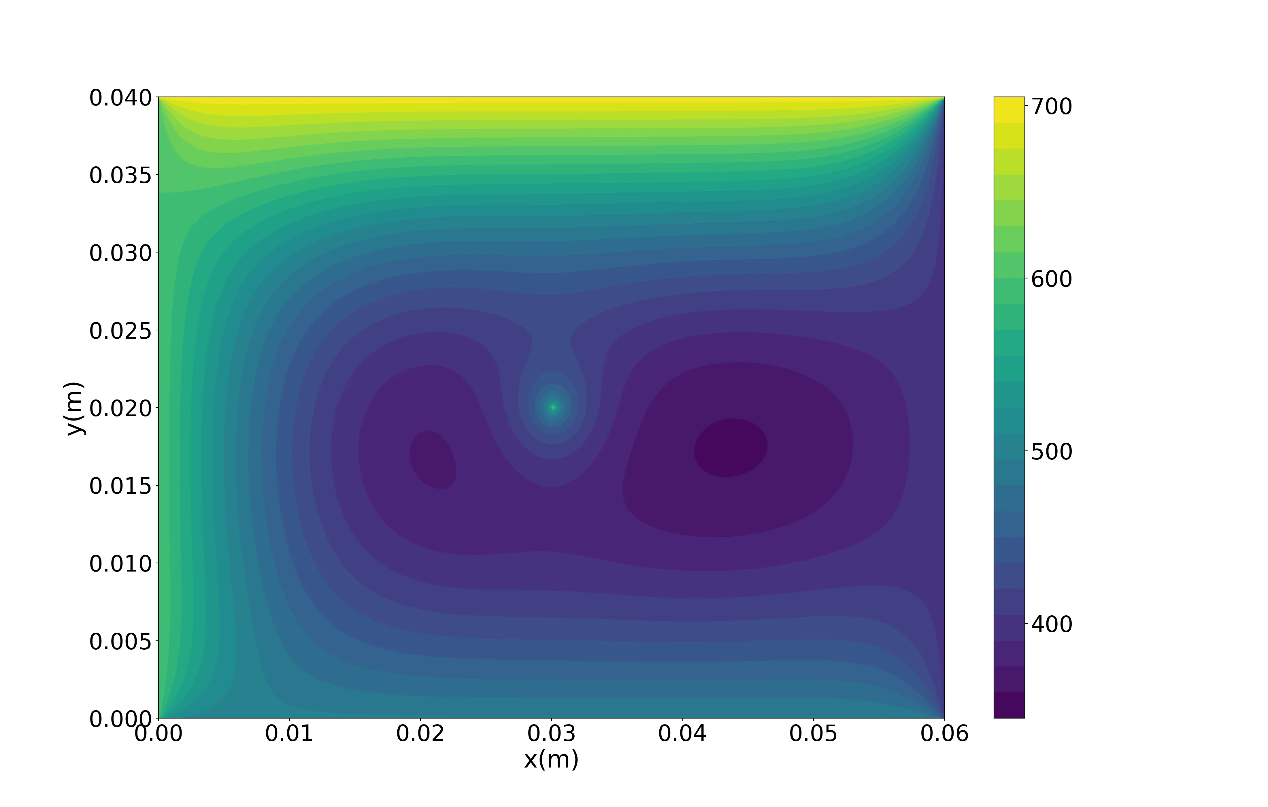
Here is the output of the Python script:

Contours of temperature in the rectangular plate.

Reflections and Takeaways

Having finished this class, you should now be able to answer the following questions:

1. What is the 2D Poisson equation?
2. Why is the 2D Poisson equation relevant for CFD applications?
3. What are the important steps towards the numerical solution of the 2D Poisson equation?
4. How do I run a parallel job on the cluster?