Optimizing CFD for HPC

Learning Objectives

At the end of this class, you should be able to:

1. Run a comprehensive scaling and determine the most efficient HPC usage
2. Determine the optimal HPC system for a given CFD problem
3. List of strategies to optimize a CFD code in HPC

Time to complete: 90 min

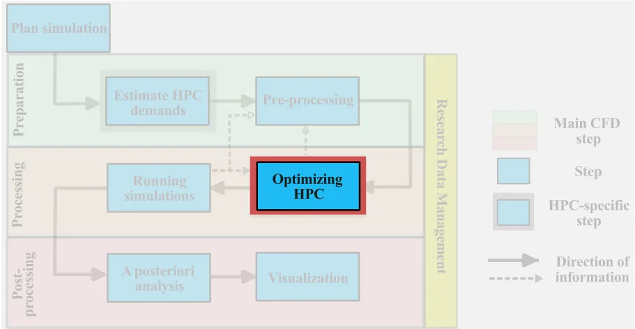
In the previous classes, we planned the simulations, estimated the HPC costs, and preprocessed the simulation. Now, we will turn our attention to optimizing the usage of HPC resources. In this section, for a given CFD simulation and code, the objective is to develop strategies to most effectively use the available HPC resources. We will assume an end-user approach to the CFD code, therefore, we will not cover topics that would force us to look ‘under the hood’ (into the code).

Assessing scalability of the code

To optimally utilize HPC resources, the CFD solver must be parallelizable and scalable. That is to say, by increasing the number of compute cores, we reduce the overall wall-clock time for a given problem. This speedup is achieved if each processor is able to complete computational tasks independently from the other. To quantify the parallel performance of a CFD problem on a CFD code, we define two types of scaling: strong scaling and weak scaling. Each is presented in this section.

Strong scaling

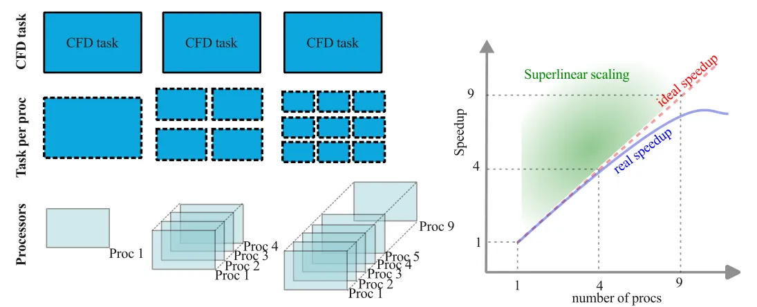
Strong scaling, also referred to as Amdahl’s law, quantifies the expected speedup with increasing number of computational processors for a fixed-sized computational task. For a fixed task, such as a CFD simulation, increasing the number of parallel processes results in a decrease in the workload per processor, thus, this should result in a reduction of wall clock time. Eventually, as the number of processors increases and the per-processor workload shrinks, the communication overhead between the processors will impact the strong scaling. Strong scaling is particularly useful for compute-bound processes (CPU-bound), which are typical of most CFD software. These tests can also help identify potential load balancing issues in the simulation.

Many tasks can be divided among processors to reduce the overall computational cost of the simulations, yet some task, let us call them ‘housekeeping’ tasks, cannot be effectively parallelized. In CFD codes, ‘housekeeping’ tasks may be tied to reading input files, checking and loading the mesh or allocating variables, which usually is most important in the initialization of the simulation. For most large-scale simulations, these poorly parallelizable tasks (usually) represent only a minimal amount of the total computational cost. Let us assume a CFD simulation is parallelizable with minimal serial housekeeping tasks, the speedup can be defined as the ratio of the time it takes (in seconds) a specific task on 1 processor () to time of the same task on processors ():

Ideal parallelizability would imply that doubling the number of processors would halve the computational wall clock time, or: . This would correspond to 100% parallel efficiency of the code, where the parallel efficiency is defined as:

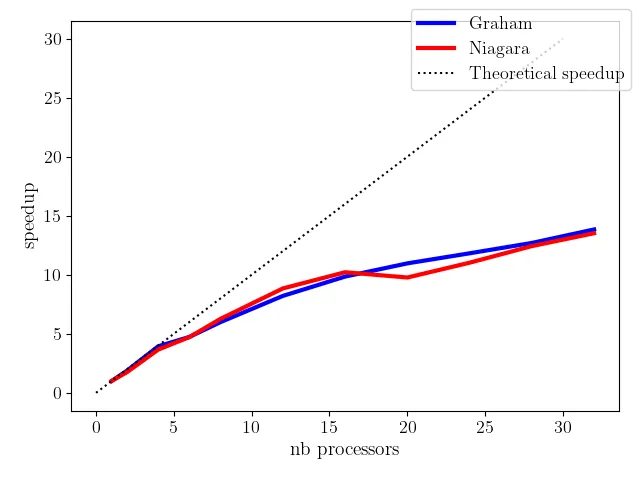
Efficiency is usually below unity, but in special cases superlinear scaling may be possible. The figure below illustrates the main points in strong scaling. It is important to keep in mind that:

• Strong scaling is code and HPC architecture dependent
• Increasing the degrees of freedom of the problem will usually improve parallel efficiency (if efficiency is bogged down by communication overhead)
• Although theoretically possible, superlinear speed up is usually rarely observed in CFD simulations

Strong scaling of a CFD code.

Weak scaling

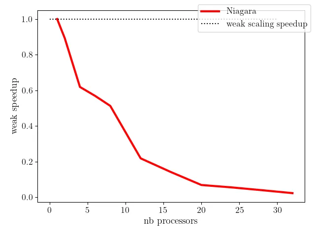
Weak scaling defines the computational efficiency of a scaled problem size with the number of processors. Weak scaling evaluates a constant per processor workload and thus provides an estimate of the approximate size of the computational task on a larger HPC system for the same wall clock time. Weak scaling is often referred to as Gustafson’s law and is a particularly useful to evaluate memory-limited applications; embarrassingly parallel problems tend to have near perfect weak scaling. As weak scaling involves increasing the computational tasks with this number of processors, this implies scaling the number of grid points with the number of processors, thus representing a much more involved scaling test compared to strong scaling.

For a problem size of computed on processors, the time to complete a task is . With these definitions, we can define the weak scaling speedup as:

It is clear that the size of the computational task on the denominator (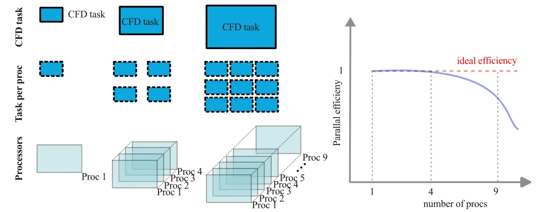) increases with the number processors, thus maintaining a constant workload on each processor. As the number of processes increases, the communication overhead also increases, reducing the weak scaling speedup. For geometrically complex problems, weak scaling is challenging, as it requires a new mesh for each number of processors. For a 2D structured mesh, we can, for example, define to be run on 1 processor. On four processors, each processor would run but the total CFD problem would be ; on 16 processors, each processor still but the total problem size is , and so on. For a comprehensive weak scaling analysis, one could conduct multiple analyses with on each processor, then on each processor, then and so forth. These multiple weak scaling results can provide a more comprehensive computational expectation of the code.

Weak scaling of a CFD code.

Scaling tests for CFD

The scaling tests are an essential component to running large-scale simulations on HPC systems. It is important that the scaling test will naturally depend on the CFD code but also, very importantly, will depend on the actual simulation and HPC system. For example, if you use a dynamic inflow boundary condition (injection of turbulence at the inlet), the local overhead in computing the inflow variable may result in a slowdown due to the processor waiting on others (load balancing issues that could impact strong scaling). As the result, a same CFD code with different operating conditions may show different scaling properties. Similarly, the same code run on two different HPC systems may also show different scaling results. Keep in mind that code performance is dependent on the architecture of the HPC system.

Tip

It is important to conduct scaling tests on:

1. A similar or identical CFD setup that you plan to run
2. The same HPC system that you plan on using

To quantify the scaling, we must have tools to measure it. Most commonly, we will use the wall-clock time in scaling test, but other quantifiable metrics may also be used. The Alliance HPC systems, we have the following command that can be used to compute the wall clock time for a given process:

[user@nia0144] /bin/time SU2_CFD MyInput.cfg

Although this provides a time to complete the simulation, this approach does not discriminate between the parallelized tasks from the ‘housekeeping’ tasks. Another approach is to take the time calculation directly from the CFD output, especially if the time is computed on a per-time-step basis.

The following list is additional considerations you want to have when conducting scaling tests on CFD code:

1. Define a consistent metric to evaluate the compute time: e.g. wall clock time to run 100 time steps with a fixed ;
2. Avoid defining times that are not consistent or dependent on the simulation: e.g., computing wall clock time to run 1 s of simulation time if is defined based on a CFL constraint;
3. Select a metric such that you minimize the importance of the serial housekeeping tasks: for example if you only compute 5 time steps, yet the initialization takes up about 25% of the total time, you will have an incorrect assessment of the scaling;
4. Scaling is solver and hardware specific: scaling test on different architecture will give different results;
5. Use a simulation that is most representative of the actual run you plan on conducting;
6. Ideally, run multiple independent runs per job size and average the results;
7. Do not run on a shared node as utilization may impact scaling;

Let us do an example.

Example: Why do I need a scaling test on my specific case?

We often face the temptation of relying on someone else’s scaling or published scaling results to avoid the process of conducting our own scaling analysis. But it is important to investigate the scaling on a problem that is as close to the actual large-scale simulation as possible.

Let us do an example: here we conduct two scaling tests on OpenFoam using two different solvers and different problems (including of mesh size). The solvers are:

• rhoCentralFoam: Density-based compressible flow solver based on central-upwind schemes of Kurganov and Tadmor
• pimpleFoam: is a pressure-based solver designed for transient simulations of incompressible flow

Both scaling tests are conducted on Niagara. We define a common metric for both cases and perform the scaling. The scaling results are listed below

rhoCentralFoam

Proc	Time (s)	Strong scaling
1	65.81	1.00
2	34.56	1.90
4	16.36	4.02
8	8.63	7.63
16	4.92	13.38
32	3.38	19.47
64	2.23	29.51
128	1.11	59.29

pimpleFoam

Proc	Time (s)	Strong scaling
1	595.43	1.00
2	338.7	1.76
4	162.53	3.66
6	126.15	4.72
8	95.01	6.27
12	67.36	8.84
16	58.29	10.21
20	60.96	9.77
24	54.02	11.02
28	47.9	12.43
32	44.04	13.52

Compiling both strong scaling tests on the same plot, we see a drastic difference in efficiency.

Comparison of the scaling results of two solvers in OpenFoam.

With 16 processors, the efficiency is an acceptable 84% using rhoCentralFoam, but with pimpleFoam, the efficiency drop to 64% which is not very good.

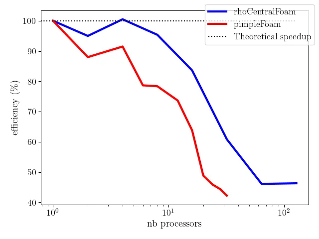
Always conduct scaling tests on the problem as close as possible to the problem you wish to scale up!

As the scaling tests require many small steps, it is possible to automate the scaling tests using bash scripts. The following example can automate a strong scaling test in OpenFoam (you need to be on an interactive node!).

Example of a bash script for strong scaling tests

strongscalingTest.sh

#!/bin/bash
#This script assumes that you've
#1)resourse allocated via commands:
#       debugjob --clean (niagara)
#       salloc -n 32 --time=1:00:0 --mem-per-cpu=3g (graham, narval ...)
#2)loaded the modules:
#       module load CCEnv StdEnv/2023  gcc/12.3  openmpi/4.1.5 openfoam/v2306 gmsh/4.12.2 (niagara)
#       module load StdEnv/2023  gcc/12.3  openmpi/4.1.5 openfoam/v2306 gmsh/4.12.2 (graham, narval ...)

# STEP1: preparing the base case
#-------------------------------
echo "STEP1: preparing the base case"
gmsh mesh/bfs.geo -3 -o mesh/bfs.msh -format msh2
gmshToFoam mesh/bfs.msh -case case
#### script to modify boundary file to reflect boundary conditions#############
  sed -i '/physical/d' case/constant/polyMesh/boundary
  sed -i "/wall_/,/startFace/{s/patch/wall/}" case/constant/polyMesh/boundary
  sed -i "/top/,/startFace/{s/patch/symmetryPlane/}" case/constant/polyMesh/boundary
  sed -i "/front/,/startFace/{s/patch/cyclic/}" case/constant/polyMesh/boundary
  sed -i "/back/,/startFace/{s/patch/cyclic/}" case/constant/polyMesh/boundary
  sed -i -e '/front/,/}/{/startFace .*/a'"\\\tneighbourPatch  back;" -e '}' case/constant/polyMesh/boundary
  sed -i -e '/back/,/}/{/startFace .*/a'"\\\tneighbourPatch  front;" -e '}' case/constant/polyMesh/boundary
  sed -i -e '/cyclic/,/nFaces/{/type .*/a'"\\\tinGroups        1(cyclic);" -e '}' case/constant/polyMesh/boundary
  sed -i -e '/wall_/,/}/{/type .*/a'"\\\tinGroups        1(wall);" -e '}' case/constant/polyMesh/boundary
#### script to modify boundary file to reflect boundary conditions#############
# STEP2: Prepare cases and run scaling test jobs
#-----------------------------------------------
echo " STEP2: Prepare cases and run scaling test jobs "
for i in 1 2 4 6 8 12 16 20 24 28 32; do
    case=bfs$i
    echo "Prepare case $case..."
    cp -r case $case
    cd $case
    sed -i "s/numberOfSubdomains.*/numberOfSubdomains ${i};/" system/decomposeParDict   #using right no. of procs
    if [ $i -eq 1 ]; then       #if serial, run AllrunSerial
       ./AllrunSerial
    else
       ./Allrun
    fi
    cd ..
done

# STEP3: Write test results to screen and file
#---------------------------------------------
echo "STEP3: Write test results to screen and file"
echo "# cores   Wall time (s):"
echo "------------------------"
echo "# cores   Wall time (s):"> SSTResults.dat
echo "------------------------">> SSTResults.dat
for i in 1 2 4 6 8 12 16 20 24 28 32; do
#for i in 1 2 4; do
    echo $i `grep Execution bfs${i}/log.pimpleFoam | tail -n 1 | cut -d " " -f 3`
    echo $i `grep Execution bfs${i}/log.pimpleFoam | tail -n 1 | cut -d " " -f 3`>> SSTResults.dat
done

Tip

A bit of planning and testing can save HPC time and effort!

Interpreting the scaling test results

Now that we have the scaling test results, we must interpret them to effectively utilize HPC systems. As most CFD codes are compute-bound, strong scaling tests are typically more relevant. Ideally, we would want to reach a compromise between parallel efficiency and the overall wall clock time.

Suppose that we have access to 32 processors and we have a CFD simulation that scales similarly to the previous example (with rhoCentralFoam). Running the simulation on 32 processors, would give us an efficiency around 60%. This would greatly under-utilize the HPC resources. In fact, running this same case on 16 processors instead of 32 would only be 31% slower. If there are, let us say, five similar simulations that need to be run, then the most effective utilization would be to run each simulation on 8 processors. This would result in a much faster throughput than running each simulation sequentially on 40 processors.

---

“The wisest are the most annoyed at the loss of (computational) time.”

-Dante Alighieri (HPC-revised)

---

Determining the optimal HPC system for a given code

Aligning the HPC system architecture for a given CFD code can help improve efficiency. Most of the time, the selection of an HPC system may be a secondary consideration, but, in other cases, when choosing between two HPC systems, it may be worth investigating.

The roofline model is a simple representation of arithmetic intensity versus performance of a code, and helps to assess the theoretical limits based on the systems architecture and memory characteristics. There are two limiting factors to the performance of a code, namely limitations on the:

1. CPU peak performance (compute-bound)
2. RAM memory bandwidth (memory-bound)

The roofline model allows a representation of those limiting characteristics. The roofline model can be mathematically defined as:

where is the hardware peak performance (FLOPS) and is the peak bandwidth. The in the above equation is the algorithmic intensity and is code dependent. The algorithmic intensity is a ratio of the number of basic operations (floating point adds and multiplies) per number of bits moved between fast and slow memory. Most CFD codes have a high algorithmic intensity, meaning they have many basic operations per cache calls. For this reason, CFD solvers are typically compute-bound in the roofline representation. Optimally, we would select a system that falls at the ridge point where the memory and computational limits intersect.

Roofline model.

Thus, when analyzing a system, we are typically interested in increasing the CPU peak performance instead of increasing the memory bandwidth. Here is an example of how the various systems can be displayed in the roofline model.

Modification of the roofline model based on the HPC characteristics.

In the above example, assuming that the computation is compute bound (high arithmetic intensity, say above 10 FLOP/bytes), the performance would be optimized with an increased CPU peak performance.

Important to keep in mind

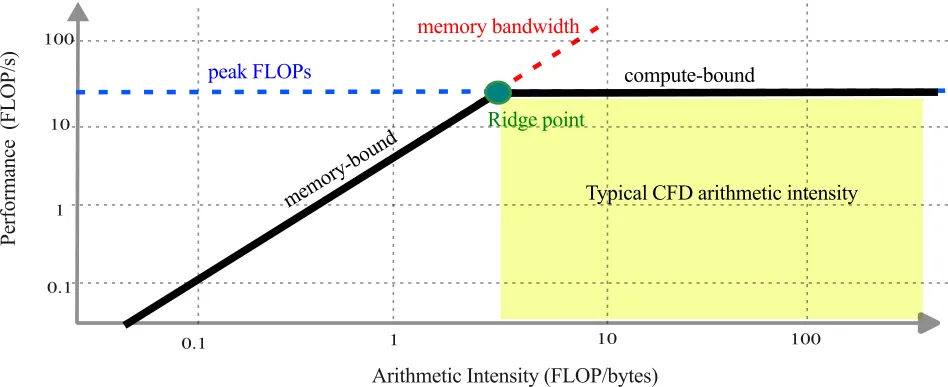
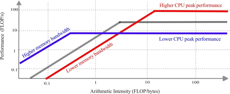
To better understand the characteristics of the processor, you can type: /proc/cpuinfo on any compute node (there is no point in checking the specs of the login node). This information provides the nominal CPU speed and cache size.

[user@<computeNode>] /proc/cpuinfo

processor  : 77
vendor_id  : GenuineIntel
cpu family  : 6
model    : 85
model name  : Intel(R) Xeon(R) Gold 6148 CPU @ 2.40GHz
stepping  : 4
microcode  : 0x2007006
cpu MHz    : 3100.195
cache size  : 28160 KB
physical id  : 1
siblings  : 40
core id    : 26
cpu cores  : 20
apicid    : 117
initial apicid  : 117
fpu    : yes
fpu_exception  : yes
cpuid level  : 22
wp    : yes

These metrics can help assess the appropriateness of a system for a CFD computation.

Strategies for effective HPC utilization

Load-balanced parallel computations

For optimal use of HPC resources, the workload should be equally distributed among all processors. When we performed the strong scaling analysis, we assumed that equally dividing the mesh among all parallel processes was equivalent to equally dividing the workload. This may not always be the case. Consider the case where the computational domain is equally divided among two processors. If, for example, the inflow condition requires the generation of synthetic turbulence (which requires a lot of ad hoc calculations), whereas the outflow is simply convected out of the domain, as shown below:

Load balancing challenges in CFD.

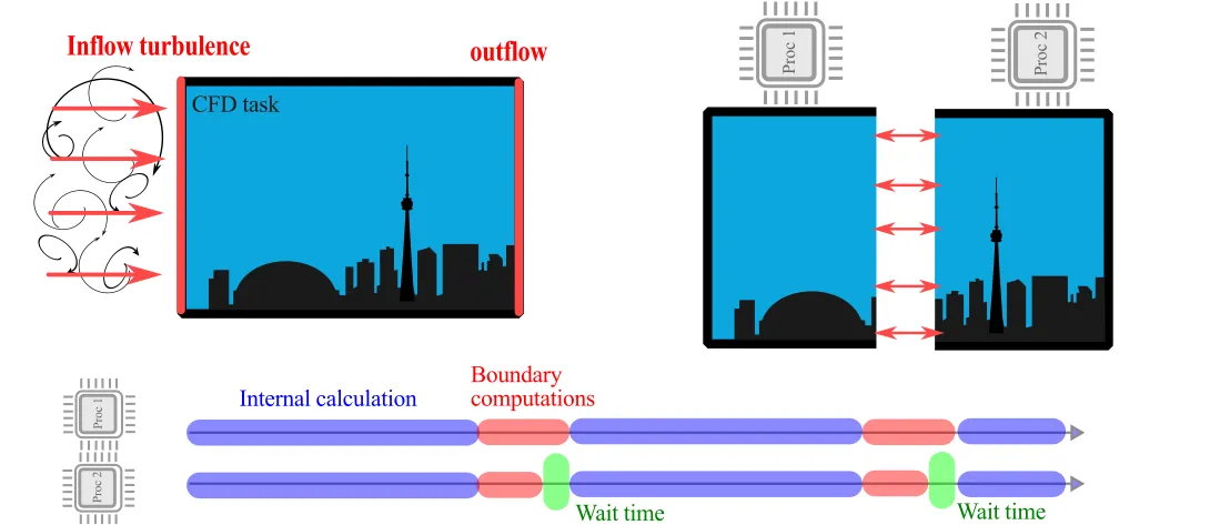
As processor 1 has the added workload of inflow conditions, processor 2 will complete its tasks sooner and have to idle while waiting for processor 1 to complete its task. For two processors, this is a completely acceptable wait time, but if we are running on 1,200 processors and only one processor delays the computation for all other 1199 processors, the load imbalance may result in significant penalty of the computation.

Load imbalances may be particularly acute in CFD as HPC systems are increasingly heterogeneous, the increased computational demands may not be equally divided; furthermore we are increasingly facing dynamic CFD workloads. The dynamic workload can be due to adaptive mesh refinement (locally increasing grid points) or through Lagrangian-based particle-laden flows, which may not be equally spread-out among the processors.

To address the combined load balancing challenges of increasingly complex codes running on heterogeneous HPC systems, dynamic load balancing can be considered, although these concepts extend beyond the scope of an introductory class. Interested readers may consult research on the topic.

Minimize communication among processors

Most modern CFD codes primarily use distributed memory parallelism using MPI processes on different physical CPU cores. As seen earlier, the interprocessor communication is often the bottleneck that limits the parallel efficiency of the code. In CFD computations, communication is necessary to compute the flux across physical MPI processes as well as averaging other operations that require information exchange (e.g. fast Fourier transforms). The decomposition of the CFD domain among the various processors is not unique and can impact the communication, and scalability of the code. Thus, one strategy, in lieu of dynamic load-balancing, is to minimize:

• Amount of information transferred
• Number of interprocessors communication links This can be done by manually dictating the decomposition of the computational domain. Let us look at an illustrative example.

Example: Minimizing communication

Consider the CFD domain comprised of grid points that can be decomposed either in four blocks of or on two dual core processors. What is the optimal decomposition? (assuming the same workload on each processor). We anticipate that communication between cores will typically have more latency than between two processors on the same chip. By looking at the amount and number of communication partners, we can anticipate that the overall communication will be more efficient with the decomposition. It is easy to comprehend how this communication problem is exacerbated when discussing the high number of cores for a 3D problem.

Optimal communication in parallel computing in CFD.

Evaluating communication of CFD simulations

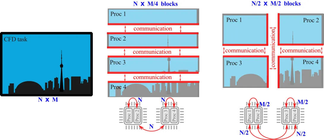
Many CFD codes rely on ParMetis (Parallel Graph Partitioning and Fill-reducing Matrix Ordering) to create high quality partitionings of very large mesh. Sometimes, the decomposition is, by default, handled directly in the code (as in SU2, although the user can also control the decomposition) other times it must be explicitly defined (as in OpenFoam). In OpenFoam, the decomposePar command decomposes the mesh and initial conditions based on the user-defined system/decomposeParDict. When running the decomposePar, the output may be helpful to assess the communication among processors. For example:

[...]

Processor 39
    Number of cells = 517259
    Number of points = 545608
    Number of faces shared with processor 19 = 5405
    Number of faces shared with processor 38 = 20216
    Number of processor patches = 2
    Number of processor faces = 25621
    Number of boundary faces = 30421

[...]

Number of processor faces = 957287
Max number of cells = 517259 (9.66634671059e-05% above average 517258.5)
Max number of processor patches = 5 (31.5789473684% above average 3.8)
Max number of faces between processors = 67248 (40.4970505188% above average 47864.35)


Number of processor faces = 1841355
Max number of cells = 258639 (0.00376987521713% above average 258629.25)
Max number of processor patches = 5 (26.582278481% above average 3.95)
Max number of faces between processors = 65100 (41.4175973672% above average 46033.875)

In the above, processor 39, must communicate information to processors 19 and 38. Additionally, at the bottom of the output, we get summary information on the total number of faces shared between processors and how evenly this is divided among all the processors. By modifying the decomposition in system/decomposeParDict, a minimized communication overhead may be achieved.

Profiling CFD codes

Profiling CFD codes can help to understand the bottlenecks in the code and provide hints about potential improvements that can improve code efficiency on HPC systems. The profiling of CFD codes on HPC systems requires more advanced computational knowledge than expected in this introductory course. The interested reader can consult the Scalasca profiler that is loaded on the Canadian clusters.

CFD-specific ideas to speed up simulations

Although improving the load-balancing and minimizing communication can speed up the simulation, the greatest speedup potential lies in the actual parameters and modelling within the simulations. Here are CFD-specific considerations that can help speed up a CFD computation:

Investigate and adjust the mesh

Looking at the preliminary results, we can identify the regions of high CFL number that are constraining the time advancement of the simulation. Is the fine mesh resolution needed at this location? Can we coarsen these mesh without affecting the results? Big computational savings can be made since doubling the characteristic mesh size at high-CFL region can effectively halve the simulation time by doubling the allowable timestep in an explicit time advancement simulation (big savings!). In most cases, fine mesh resolution is needed to resolve the local flow gradient. As such, the user must investigate the trade-off between accuracy and computational speed. In the OpenFoam output, we can obtain useful information. In the output below, we see that the AVERAGE CFL number is 675 times smaller than the cell size that constrains the time stepping. This can help us identify potential speed-up opportunities. Can we locally increase the mesh size? Can we rearrange the mesh at these locations?

Courant Number mean: 0.00404550158114 max: 2.69641684221

Consider wall modelling strategies

If we are faced with large computational cost, in this case, the user may consider applying wall-modeling strategies, which have the benefit of greatly reducing computational costs and possibly have better control on the error of the simulation. Will the added modelling of the boundary layers negatively affect the simulation results?

Coarse-to-fine mapping

Many simulations have significant transience as the flow inside the domain adapts to the boundary conditions. In fact, much of the overall HPC costs are tied to overcoming the transience, especially in turbulent flows. Can we run a coarse simulation and ‘map’ the results to a finer mesh (using mapFields in OpenFoam, for example)? We may still need to overcome a short transience as the coarse result adapts to the finer mesh, but the overall HPC costs may be reduced.

Think through the algorithms used

Some algorithms that are very beneficial for local CFD computations can be detrimental for large HPC calculations. Two cases in point are:

• Multigrid acceleration
• Preconditioners

Both of these algorithms, which greatly speed up computations on a single core system, can become a computationally liability on large computations. Both algorithms require communication to many processors and may greatly affect the strong scaling performance of the code. Can the simulation be solved without these approaches?

Revisit meshing strategies

The meshing decisions in section 2.4 may need to be revisited. Can we save total grid points by using unstructured instead of structured mesh? Can we use a higher-order scheme (higher HPC cost but reduce grid points) to reduce the grid points?

Summative example: Scaling of the backward-facing step

Strong scaling of a CFD code.

EXAMPLE: Weak Scaling Test

[SCALING TESTS HERE]

Step-by-step process for scaling test

Show scaling on Graham, niagara, etc

Show difference in scaling

Strong scaling of a CFD code.

Weak scaling of a CFD code.

Reflections and Takeaways

Having finished this class, you should now be able to answer the following questions:

1. How do I perform a weak or strong scaling analysis?
2. How do I determine the optimal HPC system for a given code?
3. How do I effectively use HPC resources?